Tensorflow 实现 AutoEncoder (自编码) 网络
有监督的神经网络需要数据是有标注(Labeled)的,然而神经网络的应用范围并不止于此,我们可以用它来处理无标注的数据: 其中的一种就是这篇Blog中介绍的AutoEncoder(自编码)网络
- 自编码网络的结构如下图所示:
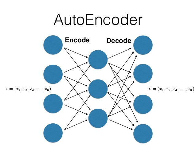
上面图中的AutoEncoder其实就是一个三层的神经网络,左侧是输入层,中间是隐藏层,最右侧为输出层。但是这个网络结果有两个特点:
- 输入层和输出层的神经单元个数是相同的;
- 隐藏层的神经单元要少于输出层。
AutoEncoder的结构为什么会有这样的特点呢?其实AutoEncoder的作用就是,将输入样本压缩到隐藏层,然后再在输出层重建样本,让输入层和输出层有如下的关系:
从上面就可以看出来,自编码网络就可以看作是,将数据压缩(压缩后的维度等于隐藏层的节点数),然后再在输出层以损失误差最小的方式将数据重建出来。
- 要注意的是输出层的取值范围在0和1之间,所以对于输入层需要进行归一化
1.导入 tensorflow 包并下载 MNIST 数据
# Import MNIST data
import tensorflow as tf
import numpy as np
import matplotlib.pyplot as plt

# Import MNIST data
from tensorflow.examples.tutorials.mnist import input_data
mnist = input_data.read_data_sets("MNIST_data/", one_hot=True)
首先准备数据,如果本地已经下载好了数据,input_data下的read_data_sets则不会重新下载数据,而是将数据加载进来。
这里用到的 tensorflow 版本为 1.0.0,其他版本没有测试。这里引入了Matplotlib用于最后结果的显示。
2.定义训练参数和网络参数
# Parameters
learning_rate = 0.01
training_epochs = 20
batch_size = 256
display_step = 1
examples_to_show = 10

# Network Parameters
n_hidden_1 = 256 # 1st layer num features
n_hidden_2 = 128 # 2nd layer num features
n_input = 784 # MNIST data input (img shape: 28* 28)
参数说明:
- 训练时的参数,比如学习率、训练轮数、训练批次的大小和结果显示的步长
- 网络结构参数,隐藏层的单元数、网络的输入和输出数。这里其实用到了两个隐藏层,先将输入数据(784维)通过hidden layer1压缩到了256维,然后再通过hidden layer2将数据从256维压缩到了128维,输出是相反的过程。
3.定义模型的输入和权重、偏置
# tf Graph input (only pictures)
X = tf.placeholder("float", [None, n_input])

weights = {
    "encoder_h1": tf.Variable(tf.random_normal([n_input, n_hidden_1])),
    "encoder_h2": tf.Variable(tf.random_normal([n_hidden_1, n_hidden_2])),
    "decoder_h1": tf.Variable(tf.random_normal([n_hidden_2, n_hidden_1])),
    "decoder_h2": tf.Variable(tf.random_normal([n_hidden_1, n_input])),
}

biases = {
    "encoder_b1": tf.Variable(tf.random_normal([n_hidden_1])),
    "encoder_b2": tf.Variable(tf.random_normal([n_hidden_2])),
    "decoder_b1": tf.Variable(tf.random_normal([n_hidden_1])),
    "decoder_b2": tf.Variable(tf.random_normal([n_input])),
}
这里用 placeholder 来装载输入变量,格式为 float
- x: 训练数据集,维度为 _ * 784 (MNIST 的图像shape 为 28*28)
因为AutoEncoder是一种无监督的方式,所以并不需要输入数据的Label。
对于权重和偏置就都通过tf.Variable来定义,并进行正态随机初始化。
4.定义Encoder和Decoder
# Building the encoder
def encoder(x):
    # Encoder Hidden layer with sigmoid activation #1
    layer_1 = tf.nn.sigmoid(tf.add(tf.matmul(x, weights['encoder_h1']),
                                   biases['encoder_b1']))
    # Encoder Hidden layer with sigmoid activation #2
    layer_2 = tf.nn.sigmoid(tf.add(tf.matmul(layer_1, weights['encoder_h2']),
                                   biases['encoder_b2']))
    return layer_2

# Building the decoder
def decoder(x):
    # Decoder Hidden layer with sigmoid activation #1
    layer_1 = tf.nn.sigmoid(tf.add(tf.matmul(x, weights['decoder_h1']),
                                   biases['decoder_b1']))
    # Decoder Hidden layer with sigmoid activation #2
    layer_2 = tf.nn.sigmoid(tf.add(tf.matmul(layer_1, weights['decoder_h2']),
                                   biases['decoder_b2']))
    return layer_2
Encoder和Decoder和之前的文章中定义的网络没有什么不同,只是这里对每层的输出用sigmoid函数进行激励。
5.定义模型的损失函数和优化方式
# Construct model
encoder_op = encoder(X)
decoder_op = decoder(encoder_op)

# Prediction
y_pred = decoder_op
# Targets (Labels) are the input data
y_true = X

# Define loss and optimizer, minimize the suqared error
cost = tf.reduce_mean(tf.pow(y_true - y_pred, 2))
optimizer = tf.train.RMSPropOptimizer(learning_rate).minimize(cost)

# Initializing the variables
init = tf.global_variables_initializer()
这里使用Mean Square Loss,优化器使用RMSPropOptimizer。
6.模型训练、测试
# Launch the graph
# Using InteractiveSession ( more convenient while using Notebooks)
sess = tf.InteractiveSession()
sess.run(init)

total_batch = int(mnist.train.num_examples/batch_size)
# Training cycle
for epoch in range(training_epochs):
    # Loop over all batches
    for i in range(total_batch):
        batch_xs, batch_ys = mnist.train.next_batch(batch_size)
        # Run optimization op (backprop) and cost op (to get loss value)
        _, c = sess.run([optimizer, cost], feed_dict={X: batch_xs})
    # Display logs per epoch step
    if epoch % display_step == 0:
        print ("Epoch:","%04d" % (epoch+1),\
               "cost=", "{:.9f}".format(c))

print ("Optimization Finished!")

# Applying encode and decode over test set
encode_decode = sess.run(
    y_pred, feed_dict={X: mnist.test.images[:examples_to_show]}
)
7.结果对比
Encoder过程其实就是将数据进行压缩,Decoder是对数据进行还原。
下面来看一下Encoder对图片进行压缩后和原始图片的对比:
